1. Introduction

Linear regression coefficients and the Pearson R correlation has long been used to quantify the relationship between dependent and independent variables [1]. However, the “ecological fallacy” has shown that linear regression and correlation coefficients based on group averages cannot be used to estimate linear regression and correlation coefficients based on individual scores [2, 3].

It may not be well known that if all possible groups are considered, in the case of sampling distributions of the mean, the Pearson R coefficient computed from the group averages is equal to the Pearson R coefficient computed from the original individual scores for one independent variable [4, 5]. We extend this result and show that the linear regression coefficients (for simple and multiple regression) and the coefficient of determination R² computed from sampling distributions of the mean (with or without replacement) are the same as the coefficient of determination and linear regression coefficients computed with the original individual           data. The sampling distributions of the mean can also be constructed using differences between two groups of different size. The result has implications for hierarchical clustering of genes. Specifically, the Pearson R coefficient can be used to measure how differential expression in one gene correlates with differential expression in a second gene.  

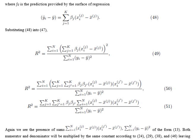
The standard error of estimate is a measure of accuracy for the surface of regression [6]. Using the coefficient of determination, we show that the standard error of estimate is reduced by the square root of the group size for sampling distributions of the mean.

In Section 1, we recall and reformulate the system of equations that are solved to determine the linear regression coefficients for individual scores. In Section 2, we prove the assertion that the same system of equations needs to be solved for sampling distributions of the mean with and without replacement or differences between two groups of sampling distributions. In Section 3, we show that the coefficient of determination is the same whether it is calculated using individual scores or all possible group averages from sampling distributions. Section 4 shows that the standard error of estimate is reduced by the square root of the group size for sampling distributions of the mean. Section 5 performs numerical simulations to illustrate these principles. Section 6 applies these results and shows that the Pearson R coefficient can be used to measure how differential expression in one gene correlates with differential expression in a second gene when the z-statistic is used.

2. Computing regression coefficients

Multiple regression requires one to compute the coefficients that minimize the sum of squares

where x⁽¹⁾, x⁽²⁾, ..., x^(K) represent K different independent variables, y is the dependent variable, and the i^th  realization of variables x^(j) and y  are x_i^(j) and y_i,  respectively, 1 ≤ i ≤ N. Note that for simple linear regression, K = 1. We recast the sum (1) in the form

where

and the coefficients are related by

To solve for β₀, we set the partial derivative of (2) with respect to β₀ to zero which yields

However

which implies that β₀ = 0. Thus one can redefine the problem of computing multiple regression coefficients (1) to be the selection of the coefficients that minimizes the sum of squares

In the matrix approach to minimizing the sum of squares which can be derived by setting the partial derivatives of (8) to zero, the system of equations in (8) is written in matrix form [8]

where

and X is a N by K matrix whose entries are:

One can solve for the multiple regression coefficients in the vector β by left multiplying (9) by the transpose X^T and solving the linear system

The elements in the square K by K matrix X^T X will be sums of the form

Similarly the entries in the K by 1 vector b ≡ X^T (y − y¯) will be sums of the form

It should be noted that for each pair of fixed indices i and j, the sum in either expression (11) or (12) can be represented using a sum of the form

In the following section, we show that if the variables x⁽¹⁾, x⁽²⁾, ..., x^(k), and y are replaced with all the elements from the sampling distributions of the mean, the system (14) is obtained

for some constant α. Moreover, we obtain a closed form for the constant α. If m is the group size and we account for order, the size of the matrix X will be N^m × K for selections with replacement and for selections without replacement. However, the resulting system (14) will still be a K × K system. Since the system (14) is equivalent to the system (10), the regression coefficients for the sampling distributions of the mean will be the same as the regression coefficients computed from the original data according to (5) for 1 ≤ j ≤ K. The equivalence of β₀^∗ follows from β₀ = 0, equation (4), and the fact that the means of the original data (y¯ and x¯^(j)) are the same as the means computed using all the elements from the sampling distributions  of the mean (with or without replacement). If we assume that there are N_p elements in the sampling distribution, this can be stated mathematically as

or

where w  can represent y  or x^(j) and The sum ∑_P is a sum over all possible index values in the sampling distribution.

3. Regression with averages

Let us create elements from the sampling distribution of the mean using elements chosen from the groups

by averaging all possible groups of size m₁ and size m₂

chosen from the sets U and V . We assume without loss of generality that m₁ ≥ m₂. The first m₂ choices are paired

while the remaining choices remain unpaired

If the selections are done without replacement, p_r ≠ p_s if r ≠ s. However, if the selections are formed with replacement, p_r can equal p_s.

Let us now replace u_p and v_p in (13) with all possible averages of m₁ and m₂ elements as shown in (18),

where

for selections with replacement and

for selections without replacement where is used to denote the exclusion of  previously chosen indices

The means of the original scores are used in (19) since they are equal to the means of the sampling distributions by (15). Note that order matters in the way the sums are written in (20-21). For example, (u₁, u₂, u₃) is considered a different choice then (u₃, u₂, u₁). Disregarding order would lead to m₁! fewer terms in (21). However the same system (14) would be generated if order was not considered for sampling distributions without replacement.

Factoring out from (19) yields

Sections 2.1 and 2.2 show that S_u¯,v¯ will be equal to a factor α times S  as defined by (13) for sampling distributions with and without replacement respectively. Section 2.3 generalizes these results to differences of two groups of sampling distibutions. In all cases, the elements of the matrix X^TX and the vector X^T(y-y¯) will be multiplied by the same factor α when elements from the sampling distributions of the mean are used.

3.1 Sampling distributions with replacement

Start with S_u¯,v¯ as defined by (23).  Since we are considering sampling distribution with replacement, the values chosen for summation indices p_i do not need to be different. We will show that

If we distribute the sums inside the parentheses in (23), two types of terms are formed. The first type of term takes the form

where the same summation index p_i is used for u_pi    and v_pi . The second type of term takes the form

where different summation indices, p_i and p_j are used.

All the terms of the form shown in (26) are zero since when the sums moved to apply directly to each term can be summed independently

However

as noted by equation (7). Thus we must only consider terms of the form (25). The sum (20) acting on can be rearranged as

and simplified to

since each sum contributes a factor of N. Multiplying the right side of (28) by m₂ to ensure all summation indices p_i, i = 1,…,m₂ are accounted for and multiplying by the factor present in (23) yields (24). One can also derive (24) using random variables and expected values.

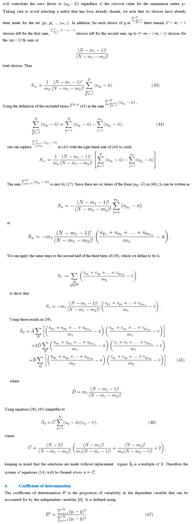
Since S_u¯,v¯  is a multiple of S  defined by (13), the system of equations (14) will be formed where when we set m = m₁ = m₂. Thus the multiple regression coefficients β computed from sampling distributions of the mean with replacement will be equal to the multiple regression coefficients computed from the original scores.

3.2 Sampling distribution without replacement

We will show that

for sampling distributions created without replacement. If we distribute the sums inside the parentheses of (23), we again distinguish between two types of terms: terms of the form and terms of the form

Choose a summation index p_i. The sum (21) applied to can be written as

where the sum with summation index p_i is placed first and the term

excludes previously chosen index values and the index value chosen for p_i. The right side of (30) can be simplified to

since the choice made for p_i in the first sum leaves N − 1 choices for the second sum, N − 2 choices for the third sum, up to N − (m₁ − 1) choices for the last sum.

Moreover there are m₂ terms similar to (30) for each summation index, p_i. Thus the terms of the form contribute

to the sum S_u¯,v¯.

We now consider terms of the form with two different summation indices p_i and p_j. The sum (21) applied to can be written as

where the sums with summation indices p_i and p_j are placed first and the term

excludes previously chosen index values and the index values chosen for p_i and p_j. Equation (32) can be simplified to

since the choice made for p_i in the first sum and p_j in the second sum leaves N − 2 choices for the third sum, N − 3 choices for the fourth sum, up to choices for the last sum. Moreover there are sums of the form (32) that can be identified when the terms in (23) are distributed. Therefore the terms of the form contribute

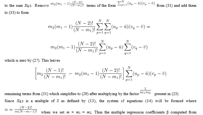sampling distributions of the mean without replacement will be equal to the multiple regression coefficients computed from the original scores.

3.3 Difference between two groups

The results in Sections 2.1 and 2.2 generalize to a difference of two groups of sampling distributions. Let m₁ be the size of Group 1 and m₂ be the size of Group 2. The two groups can be composed to allow or exclude common elements.

3.3.1 Group 1 and Group 2 can share elements

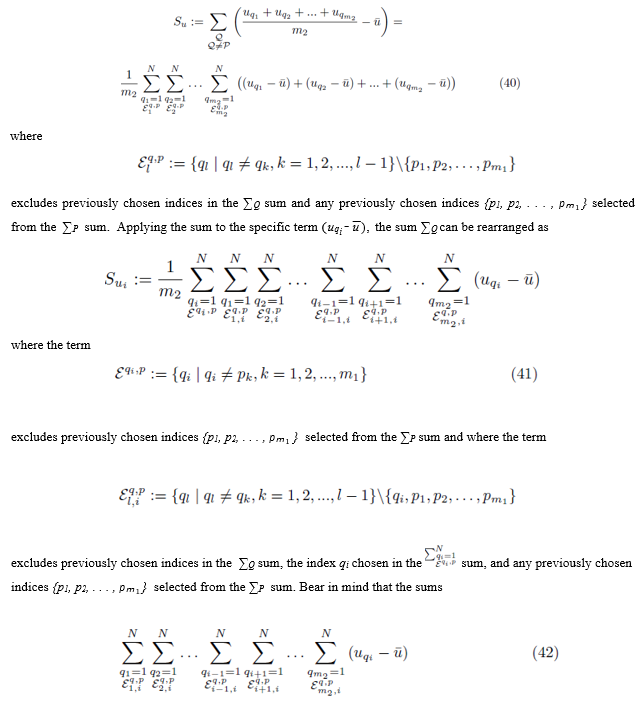
Consider the expression S_d shown in (34). The sum ∑_Q composed of m₂ iterated sums is essentially the same sum shown in either (20) or (21) except that the indexing is done with q instead of p. We first examine the case where Group 1 and Group 2 can share elements: i.e. p_i may be equal to q_j.

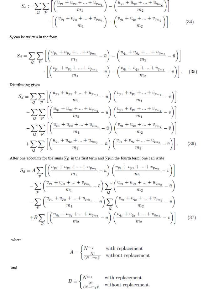
The expression for A can be derived by recognizing that N choices are available for each of the m₂ sums in ∑_Q when the selections are made with replacement. When the selections are made without replacement, there are N choices for the first sum, N – 1 choices for the second sum, up to for the m₂'th sum. The same reasoning can be used to derive the expression for B. By (16), the second and third terms in (37) are zero and can be eliminated. Using equations (24) and (29), one can simplify (37) to

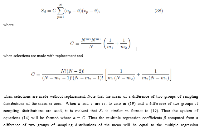coefficients β computed from a difference of two groups of sampling distributions of the mean will be equal to the multiple regression coefficients computed from the original scores.

3.3.2 Group 1 and Group 2 do not simultaneously share elements

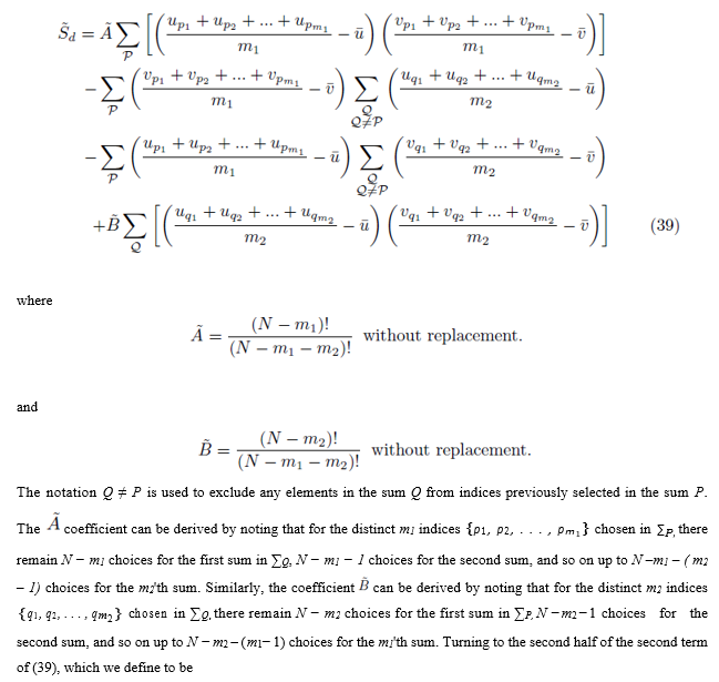
We also consider the case where Group 1 and Group 2 do not simultaneously share any elements. We assume the selections are done without replacement. Under these restrictions, one can write (36) as

5. Standard error of estimate

The standard error of estimate is a measure of accuracy for the surface of regression [7]. In this section, we show the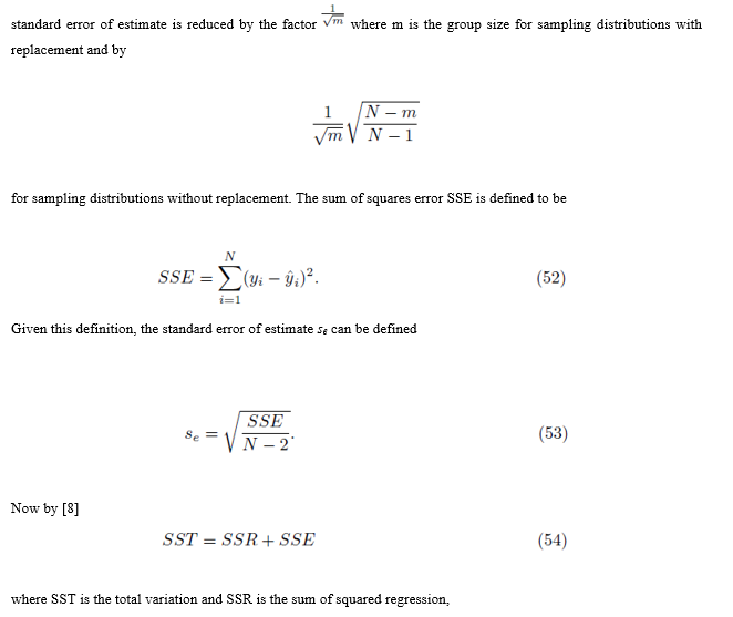

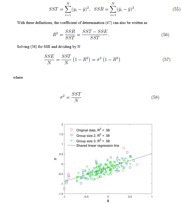
Figure 1: Original data (x_i, y_i), all elements from the sampling distributions of the mean, and the shared linear regression line. The red circles are the original 15 points, the blue squares are the averaged data of size m = 2, and the green asterisks are the averaged data of size m = 3 without replacement.

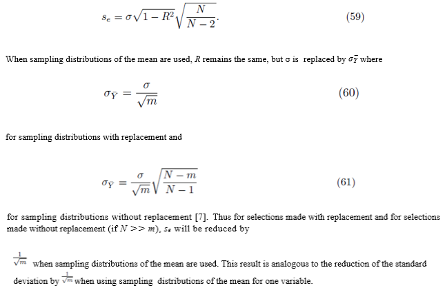
is the population variance.  Now by (53) SSE = (N − 2)s_e². Replacing SSE in (57) with (N − 2)s_e² and solving for s_e yields

6. Numerical simulations

Figure 1 plots the original data in red and all elements from the sampling distribution of the mean generated without replacement for groups of size m = 2 in blue and m = 3 in green for N = 10 original points. The original data and elements from the sampling distribution of the mean share the same regression line and  coefficient of determination R². The elements of the sampling distribution of the mean are clustered more closely about the regression line compared to the original data which is consistent with (59) and (61).

Figure 2 plots the original data in red and all elements from the sampling distribution of the mean generated without replacement for groups of size

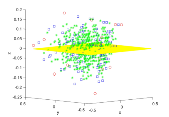
Figure 2: Original data (x_i, y_i, z_i), i = 1, 15 in red and all elements from the sampling distribution of the mean for m = 2 (blue) and m = 3 (green), and the shared linear regression plane.

m = 2 in blue and m = 3 in green for N = 15 original points. The original data and elements from the sampling distribution of the mean share the same regression plane z = .653x-712y and coefficient of determination R² = 0.76. For visualization purposes, the normal distance to the plane is plotted as the   z-coordinate and the multiple regression plane is aligned with the z = 0 plane.

Figure 3 shows the convergence of sampling distributions of the mean for{(x_i, y_i), i = 1, 2, ..., N }, N = 11 scores with Pearson correlation coefficient R = 0.35 and linear regression slope β₁ = 0.27. In the first simulation shown in black and red, elements from the sampling distributions of the mean are created using groups  of size m = 5 without replacement. In the second simulation shown in blue and green, elements from the sampling distributions of the mean are created using differences of two groups of size m₁ = 4 and m₂ = 2 without replacement. The horizontal axis plots the fraction of total selections used in the sampling distributions. There are 11⁵ = 161,051 total selections for the first simulation and 11!/5! = 332,640 total selections for the second simulation. The vertical axis plots the base 10 logarithm of the absolute difference. The absolute difference can be between either the Pearson R = 0.35 based on individual scores and the Pearson R computed from a fraction of the elements from the sampling  distributions of the mean (black and blue graphs), or between the linear regression slope β₁ = .27 based on the original scores and the slope computed using a fraction of the elements from the sampling distributions of the mean (red and green graphs). While not entirely obvious due to the density of points, all differences decrease from approximately 10⁻⁶ to less than 10⁻¹³ in the last 0.001% of the total selections. In addition, the differences do not always decrease monotonically as the fraction of total selections increase, and the differences decrease to very small values (less than 10⁻⁵) at certain points during the course of the convergence as noted by the downward spikes.

7. Gene expression and distance between genes

A useful way of organizing the data obtained from microarrays or RNA-seq data is to group together genes that exhibit similar expression patterns through hierarchical clustering. A hierarchical clustering algorithm generates a dendrogram (tree diagram). However, the algorithm requires that a distance be defined to quantify similarities in expression between two individual genes.

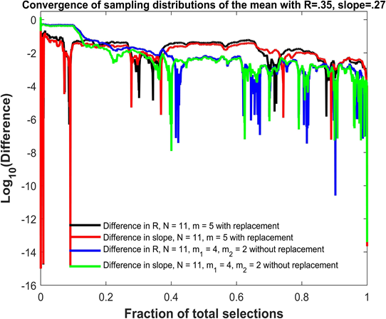
Figure 3: Convergence of the Pearson R and linear regression slope for sampling distributions of the mean.

Let A_i denote the expression level of gene A for patient i and let B_i denote the expression level for gene B for patient i, 1≤ i ≤ N. Distances between genes can be computed using many metrics [9], but two common ones are the Euclidean distance

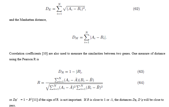
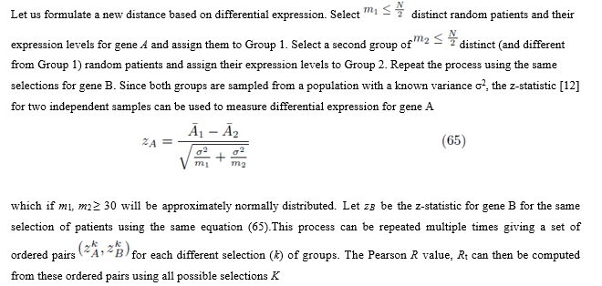
The purpose of the next section is to propose a new distance based on the differential expression of two genes. We then show the new measure of distance is the same as the Pearson R coefficient computed from the original scores (64), thus lending support to the use of the Pearson R coefficient in measuring the distance between two genes.

7.1 Formulating a new distance between two genes

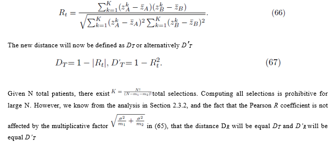
The new distance will now be defined as D_T or alternatively D′_T

8. Conclusion

We have shown that the linear regression coefficients (simple and multiple) and the coefficient of determination R² computed from sampling distributions of the mean (with or without replacement) are equal to the regression coefficients and coefficient of determination computed with the original data. This result also applies to a difference of two groups of sampling distributions of the mean. Moreover, the standard error of estimate is reduced by the square root of the group size for sampling distributions of the mean.

The result has implications for the construction of hierarchical clustering trees or heat maps which visualize the relationship between many genes. These processes require one to define a distance between two genes using their expression levels. We developed a new measure of distance based on how differential expression in one gene correlates with differential expression in a second gene using the z-statistic. We showed that the new measure is equivalent to the Pearson R coefficient computed from the original scores, thus lending support to the use of the Pearson R coefficient for measuring a distance between two genes.

Funding

This is research is supported by an Institutional Development Award (IDeA) from the National Institute of General Medical Sciences of the National Institutes of Health under grant number P20GM103451. The content is solely the responsibility of the author and does not necessarily represent the official views of the National Institutes of Health.

References

1. Yan X. Linear regression analysis: Theory and computing. Singapore: World Scientific (2009).
2. Robinson WS. Ecological correlations and the behavior of individuals. Int J Epidemiol 15 (2009): 351-357.
3. Goodman LA. Ecological regressions and the behavior of individuals. Am Sociol Rev 18 (1953): 663-664.
4. Kenney JF. Mathematics of statistics, Part Two (1947).
5. Pearson K. On the probable errors of frequency constants. Biometrika 9 (1913): 1-10.
6. Pagano R. Understanding statistics in the behavioral sciences, 10th ed. Belmont, California: Wadsworth Publishing (2012).
7. Sullivan M III. Fundamentals of statistics, 3rd ed. New York: Pearson (2010).
8. Walpole RE and Myers RH. Probability and statistics for engineers and scientists, 3rd ed. New York: MacMillan Publishing Company (1985).
9. D’haeseleer P. How does gene expression clustering work? Nat Biotechnol 23 (2005): 1499-1501.
10. Quackenbush J. Computational analysis of microarray data. Nat Rev Genet 2 (2003): 418-427.
11. Eisen MB, Spellman PT, Brown PO, et al. Cluster analysis and display of genome-wide expression patterns. Proc Natl Acad Sci USA 95 (1998): 14863-14868.
12. Triola MF. Elementary statistics using the TI-83/84 Plus calculator, 3rd ed. New York: Addison-Wesley (2011).