Classification of E. coli Colony with Generative Adversarial Networks, Discrete Wavelet Transforms and VGG19
Article Information
Pappu Kumar Yadav1*, Thomas Burks1, Kunal Dudhe2, Quentin Frederick1, Jianwei Qin3, Moon Kim3, and Mark A Ritenour4
1Department of Agricultural and Biological Engineering, P.O. Box 110570, University of Florida, Gainesville, FL 32611-0570, USA
2Department of Computer and Information Science and Engineering, University of Florida, Gainesville, Fl 32611-0570, USA
3USDA/ARS Environmental Microbial and Food Safety Laboratory, Beltsville Agricultural Research Center, Beltsville, MD 20705, USA
4Department of Horticultural Sciences, 2199 South Rock Road, University of Florida, Fort Pierce, FL 34945-3138, USA
*Corresponding Author: Pappu Kumar Yadav, Department of Agricultural and Biological Engineering, P.O. Box 110570, University of Florida, Gainesville, FL 32611-0570, USA
Received: 09 July 2023; Accepted: 18 July 2023; Published: 28 July 2023
Citation: Pappu Kumar Yadav, Thomas Burks, Kunal Dudhe , Quentin Frederick, Jianwei Qin, Moon Kim, and Mark A. Ritenour. Classification of E. coli colony with generative adversarial networks, discrete wavelet transforms and VGG19. Journal of Radiology and Clinical Imaging. 6 (2023): 146-160.
Share at FacebookAbstract
The transmission of Escherichia coli (E. coli) bacteria to humans through infected fruits, such as citrus, can lead to severe health issues, including bloody diarrhea and kidney disease (Hemolytic Uremic Syndrome). Therefore, the implementation of a suitable sensor and detection approach for inspecting the presence of E. coli colonies on fruits and vegetables would greatly enhance food safety measures. This journal article presents an evaluation of SafetySpect's Contamination, Sanitization Inspection, and Disinfection (CSI-D+) system, comprising an UV camera, an RGB camera, and illumination at two fluorescence excitation wavelengths: ultraviolet C (UVC) at 275 nm and violet at 405 nm. To conduct the study, different concentrations of bacterial populations were inoculated on black rubber slides, chosen to provide a fluorescence-free background for benchmark tests on E. coli-containing droplets. A VGG19 deep learning network was used for classifying fluorescence images with E. coli droplets at four concentration levels. Discrete wavelet transforms (DWT) were used to denoise the images and then generative adversarial networks (StyleGAN2-ADA) were used to enhance dataset size to mitigate the issue of overfitting. It was found that VGG19 with SoftMax achieved an overall accuracy of 84% without synthetic datasets and 94% with augmented datasets generated by StyleGAN2-ADA. Furthermore, employing RBF SVM increased the accuracy by 2% points to 96%, while Linear SVM enhanced it by 3% points to 97%. These findings provide valuable insights for the detection of E. coli bacterial populations on citrus peels, facilitating necessary actions for decontamination
Keywords
Discrete wavelet transform; Fluorescence images; E. coli; Food safety; StyleGAN2-ADA; Support vector machine (SVM); VGG19.
Discrete wavelet transform articles; Fluorescence images articles; E. coli; Food safety articles; StyleGAN2-ADA articles; Support vector machine (SVM) articles; VGG19 articles
Discrete wavelet transform articles Discrete wavelet transform Research articles Discrete wavelet transform review articles Discrete wavelet transform PubMed articles Discrete wavelet transform PubMed Central articles Discrete wavelet transform 2023 articles Discrete wavelet transform 2024 articles Discrete wavelet transform Scopus articles Discrete wavelet transform impact factor journals Discrete wavelet transform Scopus journals Discrete wavelet transform PubMed journals Discrete wavelet transform medical journals Discrete wavelet transform free journals Discrete wavelet transform best journals Discrete wavelet transform top journals Discrete wavelet transform free medical journals Discrete wavelet transform famous journals Discrete wavelet transform Google Scholar indexed journals Fluorescence images articles Fluorescence images Research articles Fluorescence images review articles Fluorescence images PubMed articles Fluorescence images PubMed Central articles Fluorescence images 2023 articles Fluorescence images 2024 articles Fluorescence images Scopus articles Fluorescence images impact factor journals Fluorescence images Scopus journals Fluorescence images PubMed journals Fluorescence images medical journals Fluorescence images free journals Fluorescence images best journals Fluorescence images top journals Fluorescence images free medical journals Fluorescence images famous journals Fluorescence images Google Scholar indexed journals E. coli articles E. coli Research articles E. coli review articles E. coli PubMed articles E. coli PubMed Central articles E. coli 2023 articles E. coli 2024 articles E. coli Scopus articles E. coli impact factor journals E. coli Scopus journals E. coli PubMed journals E. coli medical journals E. coli free journals E. coli best journals E. coli top journals E. coli free medical journals E. coli famous journals E. coli Google Scholar indexed journals Food safety articles Food safety Research articles Food safety review articles Food safety PubMed articles Food safety PubMed Central articles Food safety 2023 articles Food safety 2024 articles Food safety Scopus articles Food safety impact factor journals Food safety Scopus journals Food safety PubMed journals Food safety medical journals Food safety free journals Food safety best journals Food safety top journals Food safety free medical journals Food safety famous journals Food safety Google Scholar indexed journals StyleGAN2-ADA articles StyleGAN2-ADA Research articles StyleGAN2-ADA review articles StyleGAN2-ADA PubMed articles StyleGAN2-ADA PubMed Central articles StyleGAN2-ADA 2023 articles StyleGAN2-ADA 2024 articles StyleGAN2-ADA Scopus articles StyleGAN2-ADA impact factor journals StyleGAN2-ADA Scopus journals StyleGAN2-ADA PubMed journals StyleGAN2-ADA medical journals StyleGAN2-ADA free journals StyleGAN2-ADA best journals StyleGAN2-ADA top journals StyleGAN2-ADA free medical journals StyleGAN2-ADA famous journals StyleGAN2-ADA Google Scholar indexed journals Support vector machine articles Support vector machine Research articles Support vector machine review articles Support vector machine PubMed articles Support vector machine PubMed Central articles Support vector machine 2023 articles Support vector machine 2024 articles Support vector machine Scopus articles Support vector machine impact factor journals Support vector machine Scopus journals Support vector machine PubMed journals Support vector machine medical journals Support vector machine free journals Support vector machine best journals Support vector machine top journals Support vector machine free medical journals Support vector machine famous journals Support vector machine Google Scholar indexed journals VGG19 articles VGG19 Research articles VGG19 review articles VGG19 PubMed articles VGG19 PubMed Central articles VGG19 2023 articles VGG19 2024 articles VGG19 Scopus articles VGG19 impact factor journals VGG19 Scopus journals VGG19 PubMed journals VGG19 medical journals VGG19 free journals VGG19 best journals VGG19 top journals VGG19 free medical journals VGG19 famous journals VGG19 Google Scholar indexed journals ultraviolet C articles ultraviolet C Research articles ultraviolet C review articles ultraviolet C PubMed articles ultraviolet C PubMed Central articles ultraviolet C 2023 articles ultraviolet C 2024 articles ultraviolet C Scopus articles ultraviolet C impact factor journals ultraviolet C Scopus journals ultraviolet C PubMed journals ultraviolet C medical journals ultraviolet C free journals ultraviolet C best journals ultraviolet C top journals ultraviolet C free medical journals ultraviolet C famous journals ultraviolet C Google Scholar indexed journals generative adversarial networks articles generative adversarial networks Research articles generative adversarial networks review articles generative adversarial networks PubMed articles generative adversarial networks PubMed Central articles generative adversarial networks 2023 articles generative adversarial networks 2024 articles generative adversarial networks Scopus articles generative adversarial networks impact factor journals generative adversarial networks Scopus journals generative adversarial networks PubMed journals generative adversarial networks medical journals generative adversarial networks free journals generative adversarial networks best journals generative adversarial networks top journals generative adversarial networks free medical journals generative adversarial networks famous journals generative adversarial networks Google Scholar indexed journals Style generative adversarial networks-adaptive discriminator augmentation articles Style generative adversarial networks-adaptive discriminator augmentation Research articles Style generative adversarial networks-adaptive discriminator augmentation review articles Style generative adversarial networks-adaptive discriminator augmentation PubMed articles Style generative adversarial networks-adaptive discriminator augmentation PubMed Central articles Style generative adversarial networks-adaptive discriminator augmentation 2023 articles Style generative adversarial networks-adaptive discriminator augmentation 2024 articles Style generative adversarial networks-adaptive discriminator augmentation Scopus articles Style generative adversarial networks-adaptive discriminator augmentation impact factor journals Style generative adversarial networks-adaptive discriminator augmentation Scopus journals Style generative adversarial networks-adaptive discriminator augmentation PubMed journals Style generative adversarial networks-adaptive discriminator augmentation medical journals Style generative adversarial networks-adaptive discriminator augmentation free journals Style generative adversarial networks-adaptive discriminator augmentation best journals Style generative adversarial networks-adaptive discriminator augmentation top journals Style generative adversarial networks-adaptive discriminator augmentation free medical journals Style generative adversarial networks-adaptive discriminator augmentation famous journals Style generative adversarial networks-adaptive discriminator augmentation Google Scholar indexed journals
Article Details
1. Introduction
The consumption of fresh vegetables and fruits has been on the rise, leading to an increased risk of foodborne disease outbreaks caused by bacterial contamination [1]. Between 1990 and 2005, fresh fruits and vegetables accounted for 12% of reported foodborne disease outbreaks in the United States [2]. Moreover, bacterial pathogens were responsible for 60% of all foodborne disease outbreaks in the United States from 1973 to 1997 [3]. Escherichia coli (E. coli) O157:H7, in particular, is a common contributor to such outbreaks. For example, multiple incidents of E. coli-related foodborne disease outbreaks were traced back to contaminated apple cider between 1991 and 1996 [4,5]. These pathogens typically originate from healthy animals and can be transmitted to fruits and vegetables through the feces of birds, domestic animals, and wild animals like deer [5-7]. Another potential source of contamination is through irrigation water that has been contaminated [8]. In a study conducted by Solomon et al. [9], it was discovered that spray-irrigation posed a higher risk of E. coli contamination in vegetable crops compared to surface irrigation methods. Citrus fruits are also susceptible to E. coli contamination, primarily through the presence of fecal matter from birds, domestic animals, and feral animals in orchards during both pre and post-harvest stages, as well as irrigation practices. Various factors, including fruit ripeness, environmental conditions, and the ability of E. coli bacteria to withstand citrus plants' metabolic processes, can significantly influence their survival and proliferation. Once these fruits are harvested and transported to processing plants, they undergo washing treatments and industrial sanitization procedures. However, despite these measures, complete eradication of E. coli bacteria cannot be guaranteed [2, 10]. In fact, if the water used at different stages of the processing plants is contaminated with E. coli bacteria, it can serve as a potential source of citrus fruit contamination. During the post-harvest handling of citrus fruits from orchards to processing plants, humans can become infected due to the release of E. coli bacterial cells from drops present on the fruit's surface [11]. These pathogens can lead to severe health issues such as hemorrhagic colitis and gastroenteritis in affected individuals [12]. Consequently, there is a pressing need for more reliable and robust technology to ensure food safety by detecting the presence of E. coli bacterial colonies on citrus fruit surfaces, particularly at processing plants. Traditional microbial testing methods involving swabbing in a laboratory setting can be time-consuming and costly [11, 13]. Therefore, an effective solution is required that offers real-time detection of bacterial drops (E. coli colonies) on citrus fruit surfaces, followed by a rapid disinfection process. Researchers have successfully utilized fluorescence imaging systems for detecting bacterial drops [14, 15]. Additionally, previous studies have shown that ultraviolet light type C (UV-C) with a wavelength below 280 nm is the most effective method for bacterial decontamination [16]. Gorji et al. [17] demonstrated the successful application of a hand-held fluorescence imaging system (CSI-D) developed by SafetySpect Inc. (Grand Forks, ND, U.S.A.) for detecting bacterial contamination on equipment and surfaces in kitchen and restaurant areas.
In this paper, which is a derivative of our previous work [18], we show the efficacy of the newer version of the system: CSI-D+ (SafetySpect Inc., Grand Forks, ND, U.S.A.) for detecting a non-pathogenic E. coli strain ATCC 35218 [19] inoculated at four different concentration levels- : 108 , 107.7, 107.4, and 107 CFU/drop in addition to the control on an inert rubber surface as well as citrus peel plugs. Gorji et al. [17] showed that by developing deep learning algorithm, it may be possible to do real-time detection of E. coli drops with fluorescence imaging system (CSI-D+) in a non-destructive way. Therefore, the overall goal of the study presented in this paper was to develop an artificial intelligence (AI) algorithm based on combination of classical machine learning: Support Vector Machine (SVM) [20] as well as modern deep learning based on convolution neural networks (CNNs) -: VGG16 [21] to detect E. coli drops on fluorescence images. The reason we chose to use CNN was because it can do automatic feature extraction which is a requirement for developing real-time detection system [22]. Similarly, in order to harness the power of both classical machine learning and CNNs, a combination of both was used in this study as it has been found in many cases that combining both of them can provide improved results [23-25]. VGG16 is a popular CNN architecture that has been successfully used in wide variety of image classification tasks [26-29]. The performance of CNN-based AI algorithms can be negatively impacted by noisy images especially in the cases of lower concentrations of E. coli bacterial drops [30]. This is why it was required to denoise fluorescence images using discrete wavelet transformation (DWT) before they were used to train the VGG19 and SVM for classification tasks. Demir and Erturk [31] were able to improve the performance of SVM for hyperspectral image classification using wavelet transform (WT). Similarly, Serte and Demirel [32] were able to show that by denoising images with WT, the classification performance of deep learning models ResNet-18 and ResNet-50 were improved. There are many families of DWT available out of which four were used in this study: Biorthogonal (bior), Reverse biorthogonal (rbio), Daubechies (db) and Symlets (sym) [30]. Hence, it was required to find the best performing family of DWT based on reconstructed denoised images and peak signal to noise ratio (PSNR) metric so that instead of using all the four, only the best performing family was used for denoising all the images. Apart from denoising the images, there was another challenge in increasing the number of image datasets for training the VGG19 and SVM as smaller datasets generally affects the generalization and robustness of CNN-based AI algorithms [33]. It was challenging to prepare large samples of inoculated E. coli drops to train the VGG19 and SVM. In the cases of data scarcity like ours, generative adversarial networks (GANs) are widely used [34-37]. An improved version of GAN known as Style generative adversarial networks-adaptive discriminator augmentation (StyleGAN2-ADA) has been shown to generate realistic synthetic images that can be used for generating larger datasets for training deep learning and machine learning models [36]. Based on their findings, we used StyleGAN2-ADA for generating larger datasets for training the VGG19 and SVM algorithms. In this study, the specific objectives were: (i) to determine the top performing family of DWT among the four (Biorthogonal (bior), Reverse biorthogonal (rbio), Daubechies (db) and Symlets (sym)) for denoising fluorescence images with E. coli drops at four different concentration levels based on PSNR metric, (ii) to generate large dataset with StyleGAN2-ADA using the reconstructed denoised images based on the top performing DWT family and (iii) to train VGG19 for classifying the fluorescence images with E. coli drops at four
2. Materials and Methods
2.1 Contamination, Sanitization Inspection, and Disinfection (CSI-D+) System
Figure 1 shows the CSI-D+ system that was used to collect fluorescence images of rubber slides as well as citrus fruit peel plugs on which E. coli cells were inoculated at nine different concentration levels. The CSI-D+ system consists of arrays of two types of light emitting diodes (LEDs): 275-nm and 405-nm, heat sink and a driver circuit for LEDs. The 275-nm LEDs are the closest UV-C type that are commercially available for bacterial decontamination [38]. The 405-nm wavelength has been found to be effective in detection of organic residues containing fluorophores which is why another set of LEDs at this wavelength range were used for fluorescence imaging purpose in the system [38]. During fluorescence imaging, the LEDs at 405-nm are sequentially turned on and off (275-nm are turned on and off for saliva and respiratory droplets) whereas the LEDs at 275-nm are turned on for 2-5 seconds during the disinfection mode. The RGB camera in the system collects responses from the fluorophores like bacterial contaminants while the
UV camera collects responses from saliva and respirator droplets.
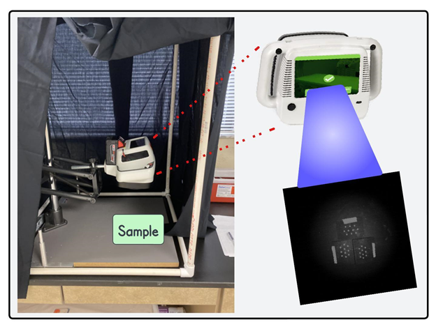
Figure 1: The new CSI-D+ system which was used to collect fluorescence images of E. coli bacterial drops inoculated on inert rubber surface.
2.2 coli Cell Preparation and Inoculation
A non-pathogenic E. coli strain (ATCC 35218) was used in this study. This E. coli strain has also been demonstrated as a surrogate for Salmonella spp. on grapefruit [19]. The E. coli strain was streaked on tryptic soy agar and incubated at 35oC for 24 h. The single colony was transferred into 10 mL of tryptic soy broth (TSB) in a test tube and incubated at 35oC for 24 h, and then 10 µL of this E. coli suspension was transferred to another 10 mL of TSB medium and incubated at 35oC for another 24 h. The E. coli suspension was centrifuged at 6000 rpm for 5 min, and the supernatant was discarded and participated E. coli cells were resuspended with sterilized distill water. Repeat this step one time. Under these conditions, E. coli cell concentrations were at about 109 cells/mL. The actual E. coli concentrations of the suspensions were confirmed and verified using dilution plate, incubation, and colony forming units (CFU) accounting method. A serial dilution of this stock suspension of E. coli (~109 cells/mL) was made to yield needed E. coli cell concentration levels such as 108.7, 108.4 and 108 cells/mL for various applications. E. coli cell suspensions at different concentration levels were transferred onto inert rubber slides or citrus fruit peel discs (2 cm in diameter) by peppering 10 individual E. coli suspension drops (10 uL each) as a group on each slide or citrus peel disc, giving a total E. coli cell concentrations at 108, 107.7, 107.4, and 107 per slide or citrus fruit peel disc, respectively. At least 4 replications were used for each E. coli cell concentration level and carrier material (rubber slide or citrus fruit peel disc). The E. coli suspensions on rubber slides or citrus fruit peel discs were dried in air with some heat applied for at least 2 h before image processing.
2.3 Image Data Preparation
The CSI-D+ system initially captured fluorescence images measuring 256 x 256 pixels in grayscale format with 8-bit depth. Each image contained three blocks of inert rubber slides, each hosting ten droplets of E. coli bacteria at identical concentration levels. Consequently, four images were obtained, each corresponding to a distinct concentration level. To introduce randomness in droplet placement and expand the dataset, background images representing rubber slides (256 x 256 pixels) were generated. A Python script was subsequently developed to extract the regions containing all 30 droplets from each image and randomly position them on the background images. The droplets were partitioned into groups ranging from 3 to 10, generating a total of 200 images measuring 256 x 256 pixels for each concentration level (800 images in total). These images were then subjected to denoising using the Wavelet Transform (WT) for further processing.
2.4 Wavelet Transform (WT)
Wavelet transform is a popular technique to remove noise from continuous or discrete signals and has been widely used for different applications [39-41]. WT decomposes a signal into wave-like oscillations that are localized in time called wavelets. This makes it advantageous over Fourier Transform which fails to capture local frequency information. As opposed to the continuous wavelet transform, DWT is the most widely used which decomposes wavelet coefficients by a factor of 2 at each level of decomposition [41]. 2D DWT was used for image data and, it was implemented by using Python package PyWavelets [42]. Four families of wavelets were used and tested in this study: Biorthogonal (bior), Reverse biorthogonal (rbio), Daubechies (db) and Symlets (sym) at decomposition level of 3. Each of the transformations generated two sets of coefficients “Approximation” and “Detail”. The Detail coefficients are of three types viz. horizontal, vertical, and diagonal. The “Approximation” coefficients were generated by passing the original image signal through low pass-low pass (LL) filters while the detail coefficients are generated by passing through high pass-low pass (HL), low pass-high pass (LH) and high pass-high pass (HH) filters. The coefficients were also used to reconstruct and obtain denoised images after 2D inverse WT (IDWT). Mathematically, DWT is defined by equation 1 [39].

Where j = 1,2...,J (maximum decomposition level), k = 1,2…N (number of wavelet coefficients), x(n) is the original signal i.e., image data in this study and ψj,k (t) is the wavelet at time ‘t’. The denoised images that were reconstructed by IDWT were analyzed based on peak signal to noise ratio (PSNR) metric. PSNR is a metric that is used to test the quality of denoised image with respect to that of the original noisy image [43,44]. Mathematically PSNR is calculated by using equation 2 [45, 46].

Where R is the maximum fluctuation in the input data type which equals to 255 for 8-bit unsigned integer data type and MSE is the mean squared error which is mathematically defined by equation 3 [45], [46].

Where M and N are number of rows and columns in an image, I and Io are original noisy and denoised images while x and y are pixel row and column indices respectively. Out of the 200 denoised images for each concentration level, 10 of them were randomly chosen and then the mean PSNR was calculated for each of the wavelet family for each concentration level. Then based on the highest value of the mean PSNR, the denoised images from the corresponding wavelet family were used for further processing.
2.5 StyleGAN2-ADA for Synthetic Dataset Generation
Generative Adversarial Networks (GANs) are ML algorithms that can generate large amount of synthetic datasets to train ML and DL algorithms for various classification and detection tasks. Among the many types of GANs, StyleGAN developed by NVIDIA researchers is quite popular due to its ability to generate realistic high quality synthetic images [34,47]. By incorporating progressive growing and adaptive instance normalization (AdaIN) at each convolution layer, StyleGAN can generate high quality synthetic images [34,48,49]. An improved version of StyleGAN called StyleGAN2 was introduced in 2019 that improved the shortcomings of the previous version by restructuring AdaIN with weight demodulation that essentially scales the feature maps based on input styles. Another improvement is done by replacing progressive growing structure with ResNet-like connections between the feature maps of low-resolution in its architecture as it introduced artifacts in generated synthetic images. Some other improvements were also made including the loss function, but it still had the challenge of training the network with smaller datasets. It was found that the discriminator part of the network could adopt to the training dataset quickly to result in overfitting issues which is why further improvement was done in the form of StyleGAN2-ADA (https://github.com/NVlabs/stylegan2-ada-pytorch) which is currently state-of-the-art GAN [34].
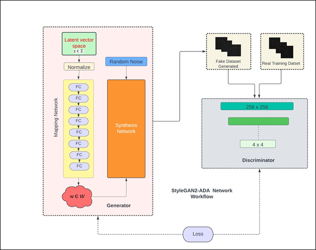
Figure: 2 Network architecture of StyleGAN2-ADA showing both generator and discriminator parts along with sample real and fake images.
Figure 2 shows a simplified network architecture of both generator and discriminator parts of StyleGAN2-ADA. The network architecture consists of a generator with a mapping and synthesis network and a discriminator. The generator is responsible for generating high dimensional synthetic/fake images from a latent space while the discriminator is responsible for classifying if the generated images are real or fake. The goal of generator is to keep improving over different iterations in such a way that the discriminator starts failing to distinguish between real and fake datasets. However, over each iteration, the discriminator keeps improving by readjusting its parameters to correctly classify fake images from the real ones. This is analogous to a min max game in which each of the two players try to outperform the other. Considering G(z) as the generator function that learns to map a latent space z ∈ N (0, I) so that it can take real image data X := x and output generated/fake image data X := xˆ. Similarly, consider D(x) as the discriminator function that represents x’s probability belonging to the real class x and not the generated/fake class xˆ. When StyleGAN2-ADA is trained, the loss of G(z) i.e., log(1-D(G(z))) is minimized while D(x) is maximized [34]. The generator uses Inception V3 as feature extractor in its network architecture [50]. The quality of generated/fake images is measured by a feature distance metric called Fréchet Inception Distance (FID). Mathematically, for univariate normal distributions X and Y, FID is given by equation 4 [51].

Where µ and σ are mean and standard deviation of X and Y. Similarly, in the context of StyleGAN2-ADA i.e., for multivariate distributions, FID is given by equation 5.

Where X and Y are multivariate feature vector distributions from real and generated/fake images i.e., activations from the Inception V3 network. µX and µY are means of X and Y respectively while Tr is the trace of the matrix and ∑X and ∑Y are covariance matrices of the feature vectors. The training parameters that were used to train the StyleGAN2-ADA are summarized in table 1.
Table 1: Training parameters that were used for StyleGAN2-ADA for the generation of synthetic E. coli datasets.
|
Parameters |
Values |
|
Seed |
600 |
|
Kimg |
2000 |
|
Learning rate |
0.0025 |
|
Snap |
50 |
2.6 6 VGG19 and support vector machine (SVM)
VGG19 is a popular CNN network widely used for varieties of image classification tasks and is an improved version of its predecessor VGG16 [52-57]. Both VGG16 and VGG19 were developed by Simonyan and Zisserman (2014) at the Visual Geometry Group at Oxford University [59]. The VGG19 was chosen for this study due to its additional three CNN layers which improves its ability for feature extraction and classification. The original architecture is designed for classifying 1000 classes by its last fully connected (FC) layer which uses SoftMax as the classifier; however, in our application, we customized it for four classes as shown in figure 3. The original network accepts input of shape 224 x 224 x 3 so it was customized to accept input of shape 256 x 256 x 3 to match the shape of our image datasets. This essentially implied that we had to train the full network without using the transfer learning approach because the pretrained weights from ImageNet [60] dataset were of the shape 224 x 224 x 3.The second and third channels of our datasets were copies of the pixel values of the first channel because of which the channel number wasn’t modified in the custom VGG19 network. VGG19 uses SoftMax classifier in its architecture as the last FC layer (Figure 3) which is a generalized version of logistic regression for multi-class classification [18, 58, 61, 62]. In our application, in the first approach, we used the SoftMax classifier and in the second approach, it was replaced by linear and non-linear (i.e., with radial basis function (RBF) kernel) support vector machine (SVM) classifiers. Assuming xi as an i-th element of the input feature vector, SoftMax function is defined as given in equation 6 [63].

Where K is equal to the number of classes, j ε [1,K], then the SoftMax classifier is defined as given in equation 7.

Where f(xi) can also be considered as the probability of xi belonging to the class j and F(xi) is the largest calculated probability of xi belonging to all the j classes. The performance of VGG19 with SoftMax classifier is measured in terms of metrices like accuracy, precision, recall, F1-score, sensitivity, and specificity as defined in equations 8-13.
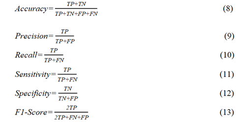
Where, TP,TN,FP, and FN represent true positives, true negatives, false positives, and false negatives respectively. SVM classifier that was used in the second approach tries to find an optimal separating hyperplane with maximum margin between classes by focusing on training data located at the edges of the distribution [64]. SVM classifier was originally designed for binary classification tasks; it however can be used for multi-class problems. The basic linear SVM classifier can be defined by equation 14 [65].

Where w and b are weights and biases, and x ε Rd is the input feature vector. 1 represents a positive class while -1 represents a negative class. A non-linear SVM uses RBF kernel function given by equation 15 [65].

Where σ is called the kernel width parameter and it plays a significant role in the performance of non-linear SVM classifier [64, 65]. The entire process from image data preparation to classification is shown by a workflow pipeline in figure 4.
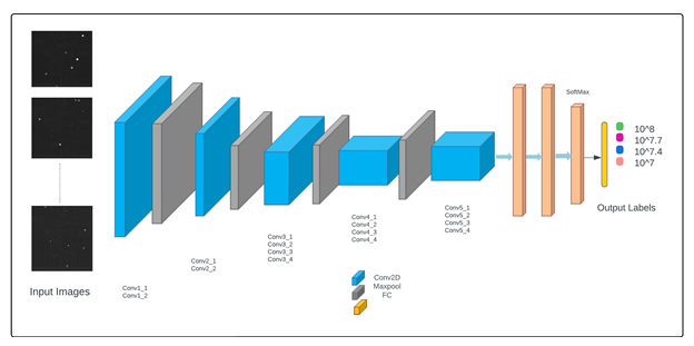
Figure 3: A customized VGG19 network architecture that was used to classify fluorescence images of E. coli bacterial population at four different concentration levels.
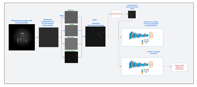
Figure 4: Workflow pipeline showing all the steps involved from image data preparation to image data classification for all the four concentration levels of E. coli bacterial populations.
3. Results and Discussion
3.1 Image Data Distribution on Rubber Surface
Once the images with randomly placed droplets containing E. coli population at four different concentration levels were generated, the distribution of pixel intensities were analyzed with 3D plots as shown in Figures 5 and 6. Figure 5 shows image data distribution of original noisy images while Figure 6 shows the same for reconstructed denoised images using IDWT. The maximum pixel intensity values remained around 100 (Figure 5) for most of the images on noisy images while it reached more than 200 (Figure 6) for the denoised images in higher concentration levels of E. coli bacterial population. This means that DWT was able to enhance pixels containing information relevant to the regions of bacterial population. The peaks in the 3D plots represent regions with E. coli bacterial population.
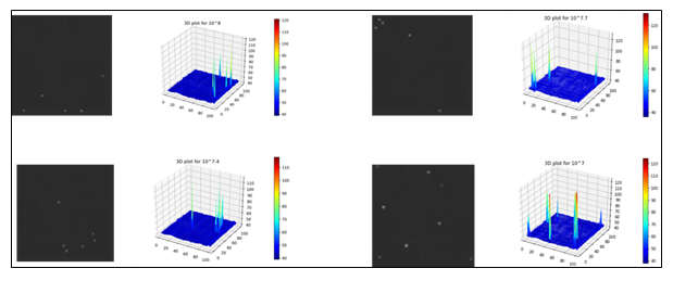
Figure 5: 3D plots of original noisy images showing regions of E. coli bacterial drops for each of the four concentration levels.
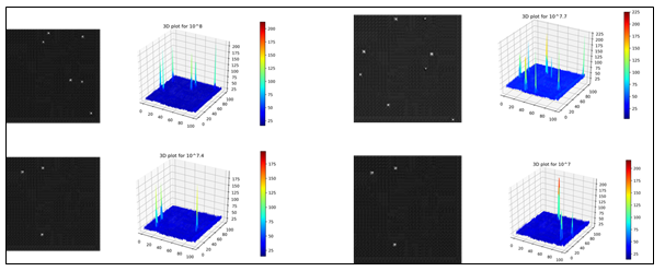
Figure 6: 3D plots of reconstructed denoised images using IDWT showing regions of E. coli bacterial population for each concentration level.
3.2 Discrete Wavelet Transform (DWT)
An example of reconstructed denoised images using DWT followed by IDWT and the corresponding distribution of pixels is shown in Figure 7. A study was conducted to determine the most effective family of DWT among the four: Biorthogonal (bior), Reverse biorthogonal (rbio), Daubechies (db) and Symlets (sym). In all the cases of four concentration levels, it was found that sym was the best performing in terms of PSNR values. An example of distribution of PSNR values obtained when tested on 10 randomly selected images belonging to 108 CFU/drop is shown in Figure 7. The mean PSNR for sym was found to be 27.84 ± 4.56 dB which is higher than the remaining three (Figure 7). Similarly, the mean PSNR values with sym for 107.7 , 107.4 and 107 CFU/drop were found to be 24.43 ± 4.61, 24.77 ± 4.42 and 25.34 ± 2.31 dB respectively.
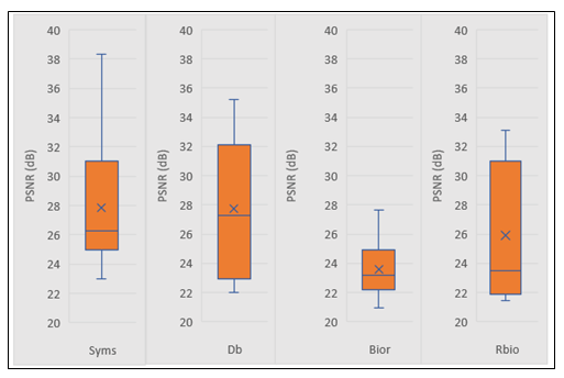
Figure 7: Box plots showing PSNR distribution of E. coli concentration at 108 CFU/drop using all the four wavelet families.
As seen in Figure 7, the second best performing family was Daubechies, which could be due to the fact that both sym and db are similar with sym modified for higher symmetry [46]. The noise reduction in highest and lowest concentration levels i.e., 108 and 107 CFU/drop were greater than the two middle concentrations levels i.e., 107.7 and 107.4 CFU/drop. This could be because in the 108 and 107 CFU/drop, the noise signals present in the higher frequency were symmetric in nature and therefore could be suppressed more effectively because of symmetric filters i.e., sym [66, 67].
3.3 Synthetic Data Using StyleGAN2-ADA
The StyleGAN2-ADA (https://github.com/NVlabs/stylegan2-ada-pytorch) network was trained on NVIDIA Tesla P100-PCIE GPU 343 (Santa Clara, CA) running Compute Unified Device Architecture (CUDA) version 11.2 and driver 344 version 460.32.03 using the Google Colab Pro+ (Google LLC., 342 Melno Park, CA) platform. The parameters used for training the network are shown in Table 1. The best FID values that were obtained for each of the four concentration levels are shown in Table 2.
Table 2: The best FID values that were obtained for each concentration level after training with StyleGAN2-ADA
|
Concentration Levels (CFU/drop) |
FID |
|
108 |
21.99 |
|
107.7 |
19.44 |
|
107.4 |
20.52 |
|
107 |
16.52 |
The plots showing changes in the FID values over different training Kimg for each concentration level are shown in Figure 8. Once the best trained network was determined based on the lowest observed FID values as shown in Table 2, synthetic images (800 for each concentration level) were generated. In this way, a total of 3,200 synthetic images were generated that were later used in combination with the sym-based reconstructed denoised images (Figure 9; 200 for each concentration level). This implied that, there were 1000 (800+200) images for each concentration level i.e., a total of 4,000 images to train the VGG19 network with SoftMax and SVM classifiers.
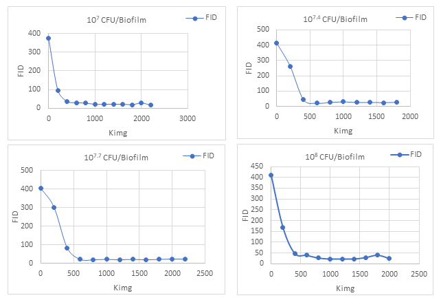
Figure 8: Plots showing FID values that were recorded every 200 Kimg during training process of StyleGAN2-ADA for all the four concentration levels.
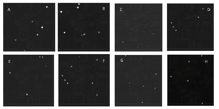
Figure 9: Images A, C, E and G are the sym-based reconstructed denoised real images for 107, 107.4, 107.7 and 108 CFU/drop concentrations respectively while the images B, D, F and H are the synthetic images generated by StyleGAN2-ADA for the four concentration levels respectively.
The generated synthetic images were realistic and very close to the real images and therefore they were used to train the VGG19 network with SoftMax and SVM classifiers for improved accuracy and better generalization as shown by Giuffrida et al. [68]and Fawakherji et al. [69].
3.4 VGG19 with SoftMax Classifier
The custom VGG19 network with SoftMax classifier was also trained on NVIDIA Tesla P100-PCIE GPU (Santa Clara, CA) using the Google Colab Pro+ (Google LLC., 342 Melno Park, CA) platform. The network was trained from scratch using adaptive learning rate method called Adadelta [70] at learning rate value of 0.001. It was trained for 50 iterations with a batch size of 8. The different types of graphs that were obtained as part of the training and validation process are shown in Figure 10.
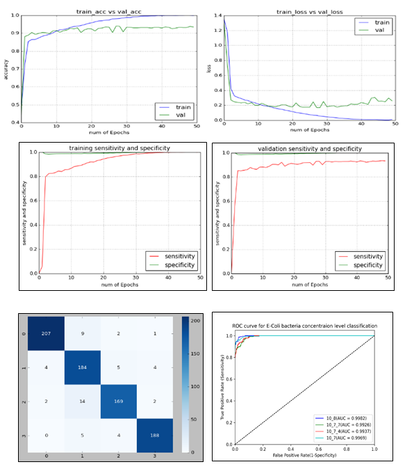
Figure 10: Accuracy, loss, sensitivity and specificity graphs for training and validation datasets including the confusion matrix and receiver operating characteristics (ROC) curves that were obtained when VGG19 was trained with SoftMax classifier.
From the accuracy and loss graphs, the network was able to reach convergence within 50 iterations and beyond this, and it showed a trend for overfitting (Figure 10). The training accuracy reached 100% while validation accuracy maxed out at 94%. Similarly, the training loss reached 0 while the validation loss remained around 0.2. The true positive rate (sensitivity) and false negative rate (specificity) both reached 100% on the training dataset while on the validation dataset, the true positive rate could reach a little over 90% whereas the false negative rate was around 100%. On both the datasets, the trained VGG19 model could classify almost perfectly the false negatives. The confusion matrix shows number of correctly and misclassified images for each concentration level. Based on this, its summary is given in Table 3 where values of precision, recall and F1-score for each concentration level are shown.
Table 3: Summary of confusion matrix showing values of precision, recall and F1-score for each concentration level after training the VGG19 network with SoftMax classifier.
|
Class Label |
Concentration(CFU/Drop) |
Precision |
Recall |
F1-Score |
|
0 |
108 |
0.97 |
0.95 |
0.96 |
|
1 |
107.7 |
0.87 |
0.93 |
0.90 |
|
2 |
107.4 |
0.94 |
0.90 |
0.92 |
|
3 |
107 |
0.96 |
0.95 |
0.96 |
It is evident that images belonging to 108 CFU/drop were most precisely classified with highest weighted accuracy i.e., F1-score. The majority of the misclassifications were observed in images belonging to 107.7 and 107.4 CFU/drop. This essentially means that the features of E. coli populations at these two concentration levels were very much like each other. The overall accuracy was found to be 94% which is 10% more than the results obtained when trained without synthetic dataset generated by StyleGAN2-ADA. This was similar to the results obtained by Liu et al. [71] in which they were able to improve grape leaf disease classification accuracy by increasing the training dataset with GANs. In addition to accuracy, areas under the ROC curve (i.e., AUC) were also used to measure the performance of the VGG19 network. This was done because it considers the entire range of threshold values between 0 and 1 and is not affected by class distribution and misclassification cost [18, 58, 62, 72, 73]. The AUC can be treated as a measure of separability and the lines belonging to a class that reaches close to the top-left corner is the most separable one. From Figure 10, the images belonging to 107 were the most separable followed by 108, 107.7 and 107.4 CFU/drop.
3.5 VGG19 with SVM Classifier
In our second approach, VGG19 was used as feature extractor and Linear and RBF SVM were used as classifiers. Dey et. al [74] had shown that SVM classifier when used with VGG19 improved pneumonia detection in chest X-rays. Similar improvement was found in early detection of Glaucoma by Raja et al [75]. In our approach, feature vectors were extracted from the last Max Pooling layer i.e., ‘block5_pool’ and then both linear and RBF SVM were trained using C parameter value as 150 and gamma parameter as ‘auto’. We also used 10 fold cross validation error estimates to determine the scores of the SVM classifiers. It was found that linear and RBF SVM classifiers were able to classify the images of all the four concentration levels with an overall accuracy of 97 ± 0.01% and 96 ± 0.01% respectively. This implied that VGG19 improved the overall classification accuracy by 3% points with linear SVM and by 2% points with RBF SVM classifiers as compared to the VGG19 with SoftMax classifier. The classification reports for both linear and RBF SVM classifiers are summarized in Tables 4 and 5.
Table 4: Classification summary report of Linear SVM using VGG19 as feature extractor
|
Class Label |
Concentration(CFU/Drop) |
Precision |
Recall |
F1-Score |
|
0 |
108 |
1.0 |
1.0 |
1.0 |
|
1 |
107.7 |
0.93 |
0.93 |
0.93 |
|
2 |
107.4 |
0.92 |
0.93 |
0.93 |
|
3 |
107 |
1.0 |
1.0 |
1.0 |
Table 5: Classification summary report of RBF SVM using VGG19 as feature extractor
|
Class Label |
Concentration(CFU/Drop) |
Precision |
Recall |
F1-Score |
|
0 |
108 |
1.0 |
1.0 |
1.0 |
|
1 |
107.7 |
0.94 |
0.93 |
0.93 |
|
2 |
107.4 |
0.92 |
0.94 |
0.93 |
|
3 |
107 |
1.0 |
1.0 |
1.0 |
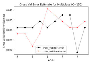
Figure 11: Plots showing cross validation error estimates for different k-folds with linear and RBF SVM.
Figure 11 shows that by adjusting k-fold values the error estimates for SVM classifiers can be adjusted. However, in most of the cases, the error estimates for linear SVM remained lower than the RBF SVM which explains the 1% higher overall accuracy. Confusion matrices for both Linear and RBF SVM classifiers are shown in Figure 12.
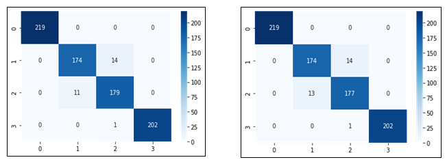
Figure 12: Confusion matrices showing number of correctly and misclassified images for all the four concentration levels represented by class labels 0,1,2 and 3 using linear (left) and RBF (right) SVM classifiers.
It is evident that there were more misclassifications for class 2 i.e., 107.4 CFU/drop using the RBF SVM than the Linear SVM. For the remaining classes, both the SVM classifiers performed the same.
4. CONCLUSION
This paper successfully demonstrates the effectiveness of the new CSI-D+ system in accurately detecting E. coli bacterial populations at various concentration levels. The use of VGG19 with Softmax classifier achieved a noteworthy accuracy of 94%. Moreover, employing RBF and Linear SVM classifiers further improved the accuracy to 96% and 97% respectively. Additionally, the study highlights the potential of discrete wavelet transform for image denoising, leading to enhanced performance of deep learning models in classification tasks. Furthermore, the utilization of synthetic datasets generated by StyleGAN2-ADA proved beneficial in improving the performance of the VGG19 model. Future work aims to implement a workflow pipeline for classifying E. coli bacterial populations on citrus fruit peels, including concentrations lower than 107 CFU/drop.
ACKNOWLEDGMENTS
We would like to extend our sincere thanks to United States Department of Agriculture-Animal and Plant Health Inspection Service (USDA-APHIS) for supporting and funding this project. We also extend our sincere gratitude and thanks towards all the reviewers and editors.
CONFLICTS OF INTEREST
The authors declare that they have no known competing financial interests or personal relationships that could have appeared to influence the work reported in this paper.
References
- RM Callejón, MI Rodríguez-Naranjo, C Ubeda, et al. “Reported foodborne outbreaks due to fresh produce in the united states and European Union: Trends and causes,” Foodborne Pathog 12 (2015): 32-38.
- JJ Luna-Guevara, MM P Arenas-Hernandez, C Martínez De La Peña, et al. “The Role of Pathogenic coli in Fresh Vegetables: Behavior, Contamination Factors, and Preventive Measures,” Int. J. Microbiol 2019 (2019): 2894328.
- CN Berger. “Fresh fruit and vegetables as vehicles for the transmission of human pathogens,” Environ. Microbiol 12 (2010): 9.
- PM Besser, RE Lett, SM Weber, et al. “An outbreak of diarrhea and hemolytic uremic syndrome from Escherichia coli O157: H7 in fresh-pressed apple cider,” JAMA - J. Am. Med. Assoc 2217 (1993): 2220.
- WJ Janisiewicz, WS Conway, MW Brown, et al. “Fate of Escherichia coli O157:H7 on fresh-cut apple tissue and its potential for transmission by fruit flies,” Appl. Environ. Microbiol 65 (1999): 1-5.
- JS Wallace, T Cheasty, and K Jones, “Isolation of Vero cytotoxin-producing Escherichia coli O157 from wild birds,” J. Appl. Microbiol 82 (1997): 399-404.
- S Kim .“Long-term excretion of shiga toxin-producing Escherichia coli (STEC) and experimental infection of a sheep with O157,” J. Vet. Med. Sci 64 (2002): 927-931.
- AJ Hamilton, F Stagnitti, R Premier, et al. “Quantitative microbial risk assessment models for consumption of raw vegetables irrigated with reclaimed water,” Appl. Environ. Microbiol 72 (2006): 3284-3290.
- EB Solomon, S Yaron, and KR Matthews. “Transmission of Escherichia coli O157:H7 from contaminated manure and irrigation water to lettuce plant tissue and its subsequent internalization,” Appl. Environ. Microbiol 68 (2002): 397-400.
- M Abadias, I Alegre, M Oliveira, et al. “Growth potential of Escherichia coli O157: H7 on fresh-cut fruits (melon and pineapple) and vegetables (carrot and escarole) stored under different conditions,” Food Control 27 (2012): 37-44.
- HT Gorji. “Deep learning and multiwavelength fluorescence imaging for cleanliness assessment and disinfection in Food Services,” Front. Sensors 3 (2022).
- LW Riley. “Hemorrhagic Colitis Associated with a Rare Escherichia coli Serotype,” N. Engl. J. Med 308 (1983): 681-685.
- K Williamson, S Pao, E Dormedy, et al. “Microbial evaluation of automated sorting systems in stone fruit packinghouses during peach packing,” Int. J. Food Microbiol 285 (2018): 98-102.
- W Jun, MS Kim, B K Cho,et al. “Microbial drop detection on food contact surfaces by macro-scale fluorescence imaging,” J. Food Eng 99 (2010): 314-322.
- AJ Lopez. “Detection of bacterial fluorescence from in vivo wound drops using a point-of-care fluorescence imaging device,” Int. Wound J 18 (2021): 626-638.
- AN Olaimat and RA Holley. “Factors influencing the microbial safety of fresh produce: A review,” Food Microbiol 32 (2012): 1-19.
- HT Gorji. “Combining deep learning and fluorescence imaging to automatically identify fecal contamination on meat carcasses,” Sci. Rep 12 (2022): 1-11.
- P Yadav .“Classifying coli concentration levels on multispectral fluorescence images with discrete wavelet transform, deep learning and support vector machine.,” in Sensing for Agriculture and Food Quality and Safety XV 1254508 (2023).
- MD Danyluk, LM Friedrich, LL Dunn, et al. “Reduction of Escherichia coli, as a surrogate for Salmonella spp., on the surface of grapefruit during various packingline processes,” Food Microbiol 78 (2018): 188-193.
- C Cortes and V Vapnik. “SupportVector Networks,” Chem. Biol. Drug Des 2 (1995): 142-147.
- K Simonyan and A Zisserman. “Very Deep Convolutional Networks for Large-Scale Image Recognition,” 3rd Int. Conf. Learn. Represent. ICLR (2015): 1-14.
- TLH Li, AB Chan and AHW Chun. “Automatic musical pattern feature extraction using convolutional neural network,” Proc. Int. MultiConference Eng. Comput. Sci (2010): 546–550.
- Z Li, X Feng, Z Wu, et al. “Classification of atrial fibrillation recurrence based on a convolution neural network with SVM architecture,” IEEE Access 7 (2019): 77849–77856.
- DA Ragab, M Sharkas, S Marshall, et al. “Breast cancer detection using deep convolutional neural networks and support vector machines,” PeerJ 2019 (2019): 1-23.
- W Wu .“An Intelligent Diagnosis Method of Brain MRI Tumor Segmentation Using Deep Convolutional Neural Network and SVM Algorithm,” Comput. Math. Methods Med., 2020 (2020).
- Y Cai, J Wu, and C. Zhang. “Classification of trash types in cotton based on deep learning,” in Chinese Control Conference (2019): 8783-8788.
- D I Swasono, H Tjandrasa and C Fathicah. “Classification of tobacco leaf pests using VGG16 transfer learning,” Proc. 2019 Int. Conf. Inf. Commun. Technol. Syst. ICTS (2019): 176-181.
- Y Tian, G Yang, Z Wang, et al. “Apple detection during different growth stages in orchards using the improved YOLO-V3 model,” Comput. Electron. Agric 157 (2019): 417-426.
- PK Yadav .“Volunteer cotton plant detection in corn field with deep learning,” in Autonomous Air and Ground Sensing Systems for Agricultural Optimization and Phenotyping VII 1211403 (2022).
- A al-Qerem, F Kharbat, S Nashwan, et al. “General model for best feature extraction of EEG using discrete wavelet transform wavelet family and differential evolution,” Int. J. Distrib. Sens. Networks 16 (2020): 3.
- B Demir and S Ertürk. “Improved hyperspectral image classification with noise reduction pre-process,” Eur. Signal Process. Conf., no. Eusipco (2008): 2-5.
- S Serte and H Demirel. “Wavelet-based deep learning for skin lesion classification,” IET Image Process 14 (2020): 720-726.
- A Sanaat, I Shiri, S Ferdowsi, et al. “Robust-Deep: A Method for Increasing Brain Imaging Datasets to Improve Deep Learning Models’ Performance and Robustness,” J. Digit. Imaging 35 (2022): 469–481.
- G Hermosilla, D I H Tapia, H Allende-Cid, et al. “Thermal Face Generation Using StyleGAN,” IEEE Access 9 (2021): 80511-80523.
- Q Zhang, H Wang, H Lu, et al. “Medical image synthesis with generative adversarial networks for tissue recognition,” Proc. - 2018 IEEE Int. Conf. Healthc. Informatics, ICHI (2018): 199-207.
- G Ahn, HS Han, MC Lee, et al. “High - resolution knee plain radiography image synthesis using style generative adversarial network adaptive discriminator augmentation,” 2021 (2023): 84-93.
- X Yi, E Walia and P Babyn. “Generative adversarial network in medical imaging: A review,” Med. Image Anal 58 (2019).
- M Sueker .“Handheld Multispectral Fluorescence Imaging System to Detect and Disinfect Surface Contamination,” (2021).
- E Cengiz, MM Kelek, Y Oguz, et al. “Classification of breast cancer with deep learning from noisy images using wavelet transform,” Biomed. Tech., vol. 67 (2022): 143-150.
- R Naga, S Chandralingam, T Anjaneyulu, et al. “Denoising EOG signal using stationary wavelet transform,” Meas. Sci. Rev 12 (2012): 46-51.
- S Shekar. “Wavelet Denoising of High-Bandwidth Nanopore and Ion-Channel Signals,” Nano Lett 19 (2019): 1090-1097.
- G R Lee, R Gommers, F Waselewski, et al. “PyWavelets: A Python package for wavelet analysis,” J. Open Source Softw 10 (2018): 21105.
- A J Santoso, L E Nugroho, GS Suparta, et al. “Compression Ratio and Peak Signal to Noise Ratio in Grayscale Image Compression using Wavelet,” Int. J. Comput. Sci. Telecommun 4333 (2011): 7-11.
- N Koonjoo, B Zhu, GC Bagnall, et al. “Boosting the signal-to-noise of low-field MRI with deep learning image reconstruction,” Sci. Rep 11 (2021): 1-16.
- SH Ismael, FM Mustafa and IT Okumus. “A New Approach of Image Denoising Based on Discrete Wavelet Transform,” Proc. - 2016 World Symp. Comput. Appl. Res. WSCAR (2016): 36-40.
- AK Yadav, R Roy, AP Kumar, et al. “De-noising of ultrasound image using discrete wavelet transform by symlet wavelet and filters,” 2015 Int. Conf. Adv. Comput. Commun. Informatics, ICACCI (2015): 1204-1208.
- T Karras, S Laine, M Aittala, et al. “Analyzing and improving the image quality of stylegan,” Proc. IEEE Comput. Soc. Conf. Comput. Vis. Pattern Recognit (2020): 8107-8116.
- X Huang and S Belongie. “Arbitrary style transfer in real-time with adaptive instance normalization,” 5th Int. Conf. Learn. Represent. ICLR (2017): 1-10.
- T Karras, T Aila, S Laine, et al. “Progressive growing of GANs for improved quality, stability, and variation,” 6th Int. Conf. Learn. Represent. ICLR (2018): 1-26.
- G Parmar, R Zhang and JY Zhu. “On Aliased Resizing and Surprising Subtleties in GAN Evaluation,” Proc. IEEE Comput. Soc. Conf. Comput. Vis. Pattern Recognit (2022): 11400-11410.
- A Thakur. “How to Evaluate GANs using Frechet Inception Distance (FID),” Weights and Biases (2023).
- SK Behera, AK Rath and PK Sethy. “Maturity status classification of papaya fruits based on machine learning and transfer learning approach,” Inf. Process. Agric 8 (2021): 244-250.
- RA Sholihati, IA Sulistijono, A Risnumawan, et al. “Potato Leaf Disease Classification Using Deep Learning Approach,” IES 2020 - Int. Electron. Symp. Role Auton. Intell. Syst. Hum. Life Comf (2020): 392-397.
- V Rajinikanth, ANJ Raj, KP Thanaraj, et al. “A customized VGG19 network with concatenation of deep and handcrafted features for brain tumor detection,” Appl. Sci., vol. 10 (2020).
- A. P. N. Kavala and R. Pothuraju, “Detection Of Grape Leaf Disease Using Transfer Learning Methods: VGG16 VGG19,” Proc. - 6th Int. Conf. Comput. Methodol. Commun. ICCMC 2022, no. Iccmc, pp. 1205–1208, 2022, doi: 10.1109/ICCMC53470.2022.9753773.
- BN Naik, R Malmathanraj and P Palanisamy. “Detection and classification of chilli leaf disease using a squeeze-and-excitation-based CNN model,” Ecol. Inform 69 (2022): 101663.
- R Sujatha, JM Chatterjee, NZ Jhanjhi, et al. “Performance of deep learning vs machine learning in plant leaf disease detection,” Microprocess. Microsyst 80 (2020): 103615.
- PK Yadav, T Burks, Q Frederick, et al. “Citrus Disease Detection using Convolution Neural Network Generated Features and Softmax Classifier on Hyperspectral Image Data,” Front. Plant Sci 13 (2022): 1-25.
- M Bansal, M Kumar, M.Sachdeva, et al. “Transfer learning for image classification using VGG19: Caltech-101 image data set,” J. Ambient Intell. Humaniz. Comput 0123456789 (2021).
- Jia Deng, Wei Dong, R. Socher, et al. “ImageNet: A large-scale hierarchical image database,” (2009): 248-255.
- Stanford, “Softmax Regression,” (2013).
- PK Yadav “Citrus disease classification with convolution neural network generated features and machine learning classifiers on hyperspectral image data,” in Autonomous Air and Ground Sensing Systems for Agricultural Optimization and Phenotyping VIII 1253902 (2023).
- Y Wu, J Li, Y Kong, et al. “Deep convolutional neural network with independent softmax for large scale face recognition,” MM (2016): 1063-1067.
- H Hasan, HZM Shafri, and M. Habshi. “A Comparison between Support Vector Machine (SVM) and Convolutional Neural Network (CNN) Models for Hyperspectral Image Classification,” in IOP Conference Series: Earth and Environmental Science 357 (2019).
- P Ghane, N Zarnaghinaghsh, and U Braga-Neto, “Comparison of Classification Algorithms Towards Subject-Specific and Subject-Independent BCI,” in International Winter Conference on Brain-Computer Interface, BCI (2021): 0-5.
- B quan Chen, J ge Cui, Q Xu, et al. “Coupling denoising algorithm based on discrete wavelet transform and modified median filter for medical image,” J. Cent. South Univ 26 (2019): 120-131.
- R Singh, RE Vasquez and R Singh. “Comparison of Daubechies, Coiflet, and Symlet for edge detection,” in Visual Information Processing VI 3074 (1997): 151-159.
- MV Giuffrida, H Scharr, and SA Tsaftaris. “ARIGAN: Synthetic arabidopsis plants using generative adversarial network,” Proc. - 2017 IEEE Int. Conf. Comput. Vis. Work. ICCVW 2018 (2017): 2064-2071.
- M Fawakherji, C Potena, I Prevedello, et al. “Data Augmentation Using GANs for Crop/Weed Segmentation in Precision Farming,” CCTA 2020 - 4th IEEE Conf. Control Technol (2020): 279-284.
- MD Zeiler. “ADADELTA: An Adaptive Learning Rate Method,” (2012).
- B Liu, C Tan, S Li, et al.“A Data Augmentation Method Based on Generative Adversarial Networks for Grape Leaf Disease Identification,” IEEE Access 8 (2020): 102188–102198.
- AP Bradley. “The use of the area under the ROC curve in the evaluation of machine learning algorithms,” Pattern Recognit 30 (1997): 1145-1159.
- XH Wang, P Shu, L Cao, et al.“A ROC curve method for performance evaluation of support vector machine with optimization strategy,” IFCSTA 2009 Proc. - 2009 Int. Forum Comput. Sci. Appl 2 (2009): 117-120.
- N Dey, YD Zhang, V Rajinikanth, et al. “Customized VGG19 Architecture for Pneumonia Detection in Chest X-Rays,” Pattern Recognit. Lett 143 (2021): 67-74.
- J Raja, P Shanmugam, and R Pitchai. “An Automated Early Detection of Glaucoma using Support Vector Machine Based Visual Geometry Group 19 (VGG-19) Convolutional Neural Network,” Wirel. Pers. Commun 118 (2021): 523–534.
